Fast Track to Aster Graphs

Aster Database includes a native graph processing engine (SQL-GR) designed to perform large-scale graph analysis on distributed graph (or network) structures. This data still lives in Aster database and, hence, is also available for processing with SQL and SQL-MR functions. In combination with SQL-GR it makes Aster a powerful platform for the best of breed approach to solving analytical problems on graphs and other network-like big data.

Aster SQL-GR functions offer wide range of graph analytics including analysis, discovery, and navigation. The names of the functions though sometimes look like a Wikipedia page on graph theory, which makes it harder answering questions like these:

• How does the network look overall?
• What is the average shortest path within network and how these values are distributed?
• What are the most prominent nodes of the network?
• What are relationships between all neighbors of a certain node?
• How are the certain nodes related to each other?

Below we demonstrate a novel approach to analyzing and working with graphs in Aster using R and toaster (version 0.5.1 or later) and show how to answer the questions like above not just simpler - but more natural.

Graph Object

Teradata Aster is relational data store utilizing relational tables for all data structures. By convention, any graph in Aster is represented using two tables:

• the vertices table must contain unique vertex key and optional columns with vertex attributes
• the edges table must contain source and target columns (as foreign keys to the vertices table) and optional columns with edge attributes

Accordingly to this convention every SQL-GR function expects at minimum the following:

• the vertex table, view or SQL query with the vertex key
• the edges table, view or SQL query with target and source keys
• if graph is directed or not
• if edges have weight attribute

To simplify and streamline graph operations toaster introduces specialized graph object toagraph in R. The toagraph object encapsulates all information about graph in Aster without requiring database connection when created. In essence, it holds all metadata necessary to call up any of Aster SQL-GR functions, so every toaster graph function will rely on it. toagraph contains the following metadata:

• vertices the name of table or view, or SQL query representing the vertices
• edges the name of table or view, or SQL query representing the edges
• directed logical flag indicating if graph is directed or not
• key the name of a unique column (key) in the vertex table or query
• source the name of a source column in the edge table or query
• target the name of a target column in the edge table or query
• vertexAttrnames vector with the names of vertex attributes (optional)
• edgeAttrnames vector with the names of edge attributes (optional)
• vertexWhere a SQL expression to filter vertices inside WHERE clause (optional)
• edgeWhere a SQL expression to filter edges inside WHERE clause (optional)

toaster Graph Functions

Designed around concrete questions about graphs and by convention starting with verb compute the 4 toaster graph functions are (as of version 0.5.1 that introduced graph features):

• computeGraph: materializes Aster graph or its subgraph as a network object in R (for more about network package see here)
• computeEgoGraph: finds and materializes the neighborhoods of given order for each of given vertices.
• computeGraphHistogram: finds distributions of various graph metrics, such as shortest path, degree, centrality measures, etc.
• computeGraphMetric: finds top vertices (or all of them) ranked by the graph metrics (degree, clustering, centrality measures, etc.)

Examples

In our examples we use Dallas Open data set that includes the graph of police officers. The edges between them were derived from the market basket analysis on police offense reports, where each report has up to two officers assigned to it. We will use the graph in all examples just by defining once this toagraph object:

policeGraphUn = toaGraph(vertices = "dallaspolice_officer_vertices", 
                         edges = "dallaspolice_officer_edges_un", 
                         directed = FALSE,
                         key = "officer", source = "officer1", target = "officer2", 
                         vertexAttrnames = c("offense_count"),
                         edgeAttrnames = c("weight"))

Next, we answer the questions above about this graph. To run examples in R you will need to install toaster and also use functions from the packages network and GGally (installed as dependencies with toaster).

How does Dallas police officer graph look?

This usually doesn't target any concrete problems but offers the comfort and guidance with bird's-eye view of the network:

netPoliceUn = computeGraph(conn, policeGraphUn)

GGally::ggnet2(netPoliceUn, node.label="vertex.names", node.size="offense_count", 
               legend.position="none", label.size=3)

# or without creating a network object
showGraph(conn, policeGraphUn, node.label="vertex.names", node.size="offense_count",
          legend.position="none", label.size=3)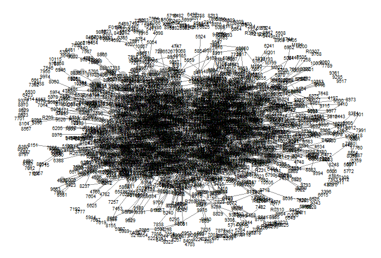

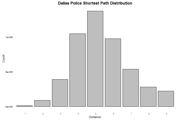
What is the average shortest path for police graph and how the shortest path values are distributed?

This is famous Six degree of separation concept (or Six Degree of Kevin Bacon) that introduces Small World graphs in social networks. computeGraphHistogram computes distributions over graph metrics, in particular, for the shortest paths calculated between all connected vertices. Then function createHistogram shows that police graph is indeed a small world network:

hshortestpathPolice = computeGraphHistogram(conn, policeGraphUn, type='shortestpath',
                                numbins = 10)
createHistogram(hshortestpathPolice, 
                title = "Dallas Police Shortest Path Distribution", 
                xlab = "Distance", ylab = "Count",
                themeExtra = theme(axis.text.x = element_text(angle = 0)))

which yields this distribution:

What are the most prominent officers based on police graph?

The question doesn't have a singular answer since "most prominent" doesn't have a singular definition in graph theory. There are different metrics that may answer the question, in particular, various centrality measures in graphs. Aster has functions for many of them, but with toaster we can retrieve top vertices for any graph metric using computeGraphMetric. For example, betweenness indicates node's centrality in a network and so if by "prominent" we mean "central" then 30 most central officers are:

topbetweenness = computeGraphMetric(conn, policeGraphUn, type='betweenness', top=30)

createTopMetricPlot(topbetweenness, 'betweenness', ylab='Betweenness', 
                    title='Top 30 Officers (Betweenness)')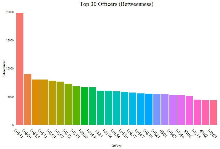

What are relationships between all neighbors for a certain officer?

Though there is no function for this in Aster it has all necessary parts to answer it. And with toaster function computeEgoGraph the assembly is not required - it was designed to build neighborhoods (ego-graphs) of given order in Aster and materialize results as subgraphs in R. Below we find the officer of the highest vertex degree (actually we find top 50 but use only the 3 highest officers to run faster) and materialize their ego-graphs of 2d order (that includes every vertex within distance of 2 and all edges between them):

library(network)
library(GGally)

# find top 50 officers their graph degree
topDegree = computeGraphMetric(conn, policeGraphUn, type="degree", top=50)

# compute ego-graphs of order 2 for top 3
topDegreeEgo = computeEgoGraph(conn, policeGraphUn, ego=as.list(as.character(topDegree$key[1:3])), order=2)

firstEgoGraph = topDegreeEgo[[1]]

# assign red color to the ego officer
firstEgoGraph %v% "color" = 
  ifelse(get.vertex.attribute(firstEgoGraph, "vertex.names") == as.character(topDegree$key[[1]]), "red", "grey")

# show resulting subgraph
ggnet2(firstEgoGraph, node.label="vertex.names", node.size="offense_count", node.color="color", legend.position="none")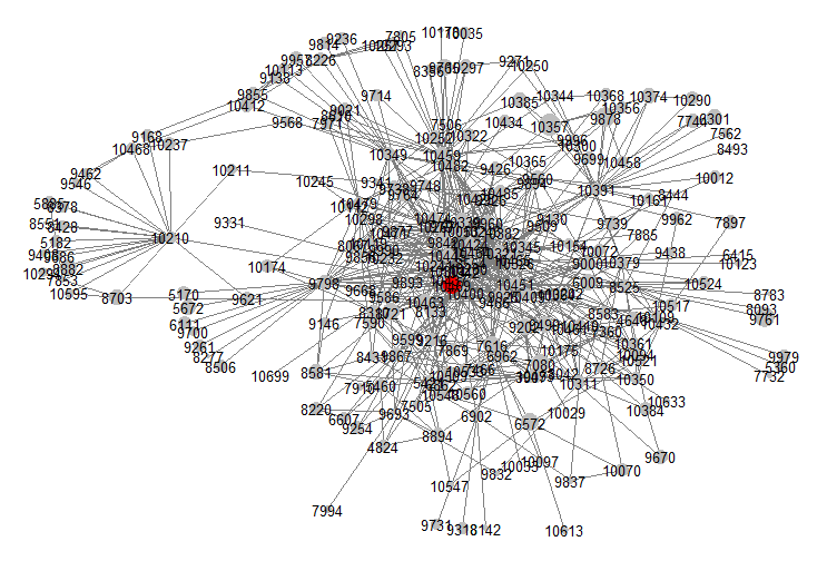

How are certain officers related to each other?

This question can usually be reduced to a problem of extracting a subgraph with given vertices. Versatility of computeGraph function makes it perfect fit to find subgraphs in Aster - in this example subgraph contains only officers having a letter in their name (key):

subGraphOfficerLetters = computeGraph(conn, policeGraphUn,  
                    v = "SELECT officer FROM dallaspolice_officer_vertices WHERE officer ~ '[A-Z].*'")

# assign colors using 1st character of officer key
subGraphOfficerLetters %v% "color" = 
  substr(get.vertex.attribute(subGraphOfficerLetters, "vertex.names"), 1, 1)

GGally::ggnet2(subGraphOfficerLetters, node.label="vertex.names", label.size=3,
               node.size="offense_count", size.cut=TRUE, node.color="color",
               palette = "Set2", legend.position="none")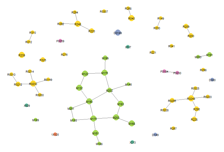

Conclusion

While Aster offers advanced graph functions the toaster's approach targets higher level tasks and problems based on graphs. It doesn't intended to replace or encapsulate all of Aster functionality but to provide effective ways to visualize and analyze graph data in R while being powered by Aster in-database performance. For example, toaster functions serve as a graph query interface to Aster database among other applications. You can find more examples on using toaster graph functions on Rpubs. We appreciate any feedback or suggestions on where to take toaster functions next.

Appendix

Function to plot top vertices by metric:

createTopMetricPlot <- function(data, metric, xlab='Officer', ylab='Degree', title) {
  p = ggplot(data) +
    geom_bar(aes_string("key", metric, fill="key"), stat='identity') +
    labs(x=xlab,y=ylab,title=title) +
    ggthemes::theme_tufte() + 
    theme(legend.position='none', 
          axis.text.x = element_text(size=16, angle = 315, vjust = 1), 
          plot.title = element_text(size=20),
          axis.ticks = element_blank())
  
  return(p)
}