Date: 2023-09-16
Version: 1.12.0
Author: Francisco Garate - fgaratesantiago (at) gmail (dot) com
Documentation: documentation_1.12.pdf
Pyliferisk is an open library written in Python for life and actuarial calculation contracts, based on commonly used methodologies among actuaries (International Actuarial Notation).
This library is able to cover all life contingencies risks (since the actuarial formulas follow the International Actuarial Notation), as well as to support the main insurance products.
This library is distributed as a single file module and has no dependencies other than the Python Standard Library, making it amazingly fast. It's compatible with both version Python 3.x and 2.7.
Additionally, the package includes several life mortality tables (pyliferisk.mortalitytables), mainly extracted from academic textbooks. Tables are added in list format. ie: SCOT_DLT_00_02_M = [0, 0.006205, 0.000328, 0.00026 ....]
First item indicates the age when table starts.
The names of the formulas follow the International Actuarial Notation and are easily guessable (qx, lx, px, w, dx, ex, Ax, Axn..), with a few exceptions regarding special characters.
The reserved variables (in addition of python language) are the following:
For the mortality assumptions in MortalityTable():
nt= The actuarial table used to perform life contingencies calculations. Syntax: nt=GKM95i= interest rate. The effective rate of interest, namely, the total interest earned in a year. Syntax: i=0.02perc= Optional variable to indicate the percentage of mortality to be applied. Syntax: perc=85 Variableperccan be omitted, in this case it will be 100 by default.
All the actuarial formulas must include a minimum of 2 variables: mt (mortality table) and x (age)
If necessary, additional variables should be included with the following order:
n (horizon in years), m (m-monthly payments), t (n-years deferred period).
Variable m can be omitted, in this case it will be 1 (annual payment) by default.
Additionally, there are two smart formulas: annuity() and A(), where the number of variables are not fixed:
annuity(nt, x, n, p, m, ['a/g', c], -d)
- mt = the mortality table
- x = the age as integer number.
- n = A integer number (term of insurance in years) or 'w' = whole-life.
- p = Moment of payment. Syntaxis: 0 = begining of each period (prepaid), 1 = end of each period (postpaid), Optional variables:
- m = Payable 'm' per year (frational payments). Default = 1 (annually)
- 'a' or 'g' = Arithmetical / Geometrical
- q = The increase rate. Syntax: ['g',q] or ['a',q]. For example, ['g',0.03] Deferring period:
- -d = The n-years deferring period as negative number.
Example 1: Print the omega (limiting age) of the both mortality tables and the qx at 50 years-old:
from pyliferisk import MortalityTable
from pyliferisk.mortalitytables import INE2004, GKM95

tariff = MortalityTable(nt=INE2004)
experience = MortalityTable(nt=GKM95, perc=85)

# Print the omega (limiting age) of the both tables:
print(tariff.w)
print(experience.w)

# Print the qx at 50 years old:
print(tariff.qx[50] / 1000)
print(experience.qx[50] / 1000)
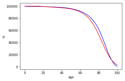
Example 2: Plotting a surviving graph:
import matplotlib.pyplot as plt
from pyliferisk import *
from pyliferisk.mortalitytables import INE2004, GKM95

tariff = MortalityTable(nt=INE2004)
experience = MortalityTable(nt=GKM95, perc=75)
x = range(0, tariff.w)
y = tariff.lx[:tariff.w]
z = experience.lx[:tariff.w]
plt.plot(x,y, color = 'blue')
plt.plot(x,z, color = 'red')
plt.ylabel('lx')
plt.xlabel('age')
Example 3:: A Life Temporal insurance for a male, 30 years-old and a horizon for 10 years, fixed annual premium (GKM80, interest 6%):
from pyliferisk import *
from pyliferisk.mortalitytables import GKM95

nt = Actuarial(nt=GKM80, i=0.06)
x = 30
n = 10
C = 1000

print(C * (Axn(nt, x, n) / annuity(nt, x, n, 0)))Once Pyhon is running, just install this library with pip install pyliferisk
It's compatible with both versions of Python: 2.7 and 3.6 Pyliferisk has no dependencies other than the Python Standard Library. That decreases the calculation runtime versus implementations under other libraries (such as Pandas).
This program is free software: you can redistribute it and/or modify it under the terms of the GNU General Public License as published by the Free Software Foundation, either version 3 of the License, or any later version.
This program is distributed in the hope that it will be useful, but WITHOUT ANY WARRANTY; without even the implied warranty of MERCHANTABILITY or FITNESS FOR A PARTICULAR PURPOSE. See the GNU General Public License for more details. The author does not take any legal responsibility for the accuracy, completeness, or usefulness of the information herein.
Contributions, feedback and suggestions for improvements are greatly appreciated.
Discussions take place on our mailing list.
http://groups.google.com/group/openactuarial (subject: pyliferisk)

